"Information contained herein is available to all without regard to
race, color, sex, or national origin."

Footnote in a paper by
Gale A. Buchanan, Director, Auburn University, Alabama
July 1985
First Things First
I am grateful to all who published emulators, firmware, software, information and what so ever
for nothing and contribute by that to democratise evolution, a bit at least.
It helped me a lot to prepare this paper, which in turn is also filed for free.
— Thank you.
Relevant Contents
- I – Theory
-
- II – Programming
-
- III – The Fine Print
- and Revision History
HP-41* Curve Fitting –
Three Special Cases of Deming Regression
In users' libraries and
program collections
you find several curve fitting solutions.
Here is another one.
* – and more.
This contribution sets its main focus on how an appropriate
Computer Algebra System
(CAS) may help to improve old programs.
If unassisted, calculus and algebra may be so time consuming
(or too error prone for tricky tasks)
to be considered as impossible.
With CAS I was able to avoid an annoying test selecting the correct one out of two eventual solutions.
No need any more to decide on concrete numbers because it is now definite and universal how to compute
the only correct solution.


Deming Regression is about curve fitting
considering different quantum of measuring errors:
- x-values taken as free of error, all errors are within y-values,
- y-values taken as free of error, all errors are within x-values,
- errors are similarly within x- and y-values,
- anything else in-between.
I regard cases 1..3 as special cases, 1 and 2 denote
the limits within a fitting line may stand
if drawn by visual judgment only, and 3 is called
Orthogonal Regression
or at odd times also "isotonic" regression.
For it the perpendicular distances from measuring point to fitting line are minimized.
The sum of the squared perpendicular distances is minimized, to be precise.
Notes:
- Case 4 is not subject of this article.
- The term curve fitting may be misleading, all considered "curves" here are straight lines
$y=\displaystyle\sum_{i=0}^1 a_i x^i \; ( x \neq 0 ) \;$ or further on $y = m \cdot x+b$,
that fit best the theory of observed readings $(x_i, y_i)$ occasionally called "dot cloud".
The results of all aforementioned cases will have the cloud's
center of mass $(\bar{x}, \bar{y})$ as origin.
If this does not meet the principle of your experiment (perhaps a different origin, (0, 0) for example)
go for a different math.
- Which CAS to pick?
- In case you'd like to redo what I describe in the following check if your CAS is capable to solve
$\displaystyle f(\bar{x})=\sum_{i=1}^{n}(x_i-\bar{x})^2$
for
${\mathrm{d}f(\bar{x})}/{\mathrm{d}\bar{x}}=0$
so to get the well-known formula of the
arithmetic average value
$\bar{x}=\displaystyle\frac{1}{n}\sum_{i=1}^n\,x_i$.
This approach is the significant LS method
(Least Squares, a method claimed by
Carl Gauss to be his idea).
Replacing $\bar{x}$ by $a$ for simpler input, Reduce returns as result of
solve(df(sum((x(k)-a)^2,k,1,n),a),a);
$\:\Rightarrow\left\{a=\displaystyle\frac{\sum_{k=1}^n\,x_k}{n}\right\}$,
what is outstanding compared to few others I've "tested" –
HP-40G,
HP-50G,
HP-Prime,
Wolfram Alpha,
and
Maxima.
("Tested" set in quotation marks as with no result by few trials I gave up quite quick,
so it's highly likely I simply had not found in reasonable time how to make it work.)
Hints:
- Since end of 2021
Reduce is accessible as an experimental online service,
at least in many browsers.
Hence there is no need to install it just for few tests, all shown examples may be tested by simple
edit/copy-edit/paste of the input from here (shown in monospaced font) to the 'Input Editor'
of Web REDUCE.
- Reduce
may display results with indexed variables,
$x_i$ instead of $x(i)$.
To get the results as shown throughout this paper
enter at first (once per session is enough)
operator (x, y); print_indexed (x, y);
"YX Regression" or L.R.
The correct term would be 'regression of y on x'.
It's the first of the above-mentioned cases, widely known as the Linear Regression
and comes with many calculator models as L.R. function – alas not with the bare HP-41.
For this model find it within chapter 'Curve Fitting' of the "HP-41C Standard Applications Handbook",
or also within chapter 'Curve Fitting' of "The HP-41 Advantage Advanced Solutions Pac".
The L.R. formulas result from applying the a. m. LS method to find $m$ and $b$ for
$\sum_{i=1}^n (y_i - (mx_i +b))^2\:\Rightarrow min$.
In case you like to do it on your own, enter in Reduce
sum((y(k)-(m*x(k)+b))^2,k,1,n); (if requested declare x and y as operators or consider
a. m. hint),
next, to get the formula for $m$ without intermediate steps, enter
order n; solve(df(sub(solve(df(ws, b), b), ws), m), m);
Note: Further on $\sum$ in formulas stands for either $\displaystyle \sum_{i=1}^n$
or $\displaystyle \sum_{k=1}^n$
"XY Regression"
The correct term would be 'regression of x on y'.
In this case it's about to minimize the horizontal distances
$\displaystyle\sum (x_i - \frac{y_i - b}{m})^2\Rightarrow min$.
Or to ease the work for Reduce:
$\displaystyle\frac{\sum (m x_i - (y_i - b))^2}{m^2}\Rightarrow min$.
Solve $\frac{\partial}{\partial b}=0$ for $b$ results in
\[\left\{b=\displaystyle\frac{-(\sum x_k)\cdot m+\sum y_k}{n}\right\}\]
Substitute with it $b$ in the formula above, then solve $\frac{\partial}{\partial m}=0$ for $m$ and get
\[\left\{m=\frac{n\left(\sum y_k^2\right)-\left(\sum y_k\right)^2}{n\left(\sum x_k\cdot y_k\right)-\left(\sum x_k\right)\cdot\left(\sum y_k\right)}\right\}\]
A
side glance to Wikipedia
shows, this is correct.
Or in concordance at least.
Look out! Some publications just swap x and y, what is amazing simple,
alas in the solution they do not swing it back again.
So far nothing to write home about, no equivocal formulas.
The first two cases, as closely related to the third, are mentioned here for completeness only.
But now to the tricky one —
Orthogonal Regression
Find $m$ and $b$ of the fitting line $y=m x+b$ so the sum of squared perpendicular distances
from metered points to that line is smallest possible.
In other words:
\[\sum \frac{(y_i - (mx_i +b))^2}{1+m^2}\Rightarrow min\]
In Reduce enter
order m, b, n; a := sum((y(k)-(m*x(k)+b))^2,k,1,n)/(1+m^2);
First get $b$ by
solve(df(a, b), b); $\Rightarrow$
$\left\{b=\displaystyle\frac{-m\left(\sum x_k\right)+\sum y_k}{n}\right\}$
what in fact is $b=\bar{y}-m\bar{x}$
and proves, as mentioned before, the line through the barycentre of the dot cloud.
Now replace $b$ in the first formula by this result and save it as new $a$:
a := sub(ws, a); $\Rightarrow$
\[a\mathrm{:=}\left(m^2 n\left(\sum x_k^2\right)-m^2\left(\sum x_k\right)^2-2mn\left(\sum x_ky_k\right)+2m\left(\sum x_k\right)\left(\sum y_k\right)+
n\left(\sum y_k^2\right)-\left(\sum y_k\right)^2\right)/\left(n\left(m^2+1\right)\right)\]
Next get $m$ by the LS method.
solve(df(a, m), m); $\Rightarrow$
\[ \left\{m=
\left(-n\sum x_k^2+n\sum y_k^2+(\sum x_k)^2-(\sum y_k)^2
\\ +\mathrm{sqrt}\left((n^2\sum x_k^2)^2-2n^2\sum x_k^2\sum y_k^2-2n\sum x_k^2(\sum x_k)^2+
2n\sum x_k^2(\sum y_k)^2+n^2(\sum y_k^2)^2+2n\sum y_k^2(\sum x_k)^2-2n\sum y_k^2(\sum y_k)^2+
4n^2(\sum x_k y_k)^2-8n\sum x_k y_k\sum x_k\sum y_k+(\sum x_k)^4+2(\sum x_k)^2(\sum y_k)^2+
(\sum y_k)^4\right)\right)/\left(2(n\sum x_k y_k-\sum x_k\sum y_k)\right)\,\mathrm{,\,}\,
\\ m=
\left(-n\sum x_k^2+n\sum y_k^2+(\sum x_k)^2-(\sum y_k)^2
\\ -\mathrm{sqrt}\left((n^2\sum x_k^2)^2-2n^2\sum x_k^2\sum y_k^2-2n\sum x_k^2(\sum x_k)^2+
2n\sum x_k^2(\sum y_k)^2+n^2(\sum y_k^2)^2+2n\sum y_k^2(\sum x_k)^2-2n\sum y_k^2(\sum y_k)^2+
4n^2(\sum x_k y_k)^2-8n\sum x_k y_k\sum x_k\sum y_k+(\sum x_k)^4+2(\sum x_k)^2(\sum y_k)^2+
(\sum y_k)^4\right)\right)/\left(2(n\sum x_k y_k-\sum x_k\sum y_k)\right)
\right\} \]
-
-
Decades ago
(skip this blah-blah...)
as student w/o CAS I gave up at this point due to lack of paper, pencil and time.
Instead of going straight on I made a program that computed both eventual solutions to decide then
which one to keep.
Similar does William M. Kolb in his "Curve Fitting for Programmable Calculators", 1982 (find a PDF of it on
W. Furlow's DVD in directory \Books).
See part II, chapter "Isotonic Linear Regression", p. 21f (page 31..32 of the PDF).
Cit: "The correct solution for most applications is given by..." End cit.
I do like programs that compute for most correctly.
My routine I found again on an old disk is accurate in any case.
It computes both, $m_1 = C + \sqrt{1+C^2}$ and $m_2 = C - \sqrt{1+C^2}$ and keeps the one
with the same sign as the value in R06.
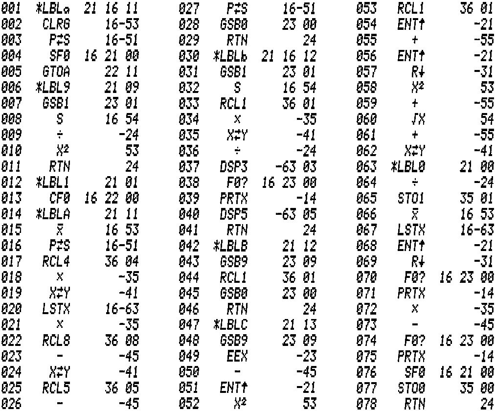
Here the snippet in question (excerpt from a longish program, § stands for $\textstyle\sum$):
Registers content:
R06 = R15 * R14 - R10 * R 12 = n * §(xy) - §x * §y = w
R07 = R15 * R11 - R10^2      = n * §(x^2) - (§x)^2 = u
R08 = R15 * R13 - R12^2      = n * §(y^2) - (§y)^2 = v
121•LBL 07  RCL 08
  RCL 07  -  RCL 06  X=0?  | if w = 0 give up
  GTO 01  RCL 06  +  /     | (v - u) / 2w = C
  ENTER^  ENTER^  X^2  1   | Y: C - sqrt(C^2 + 1) = m2
  +  SQRT  ST- Z  +        | X: C + sqrt(C^2 + 1) = m1
  RCL 06  RCL Y  *  X>0    | (w * m1) > 0? m1 : m2
  R^  MEAN  RCL Z  *  -    | b in X, m in Y, Z u. T
(32 bytes)                 | (here GTO 01 has 3 bytes)
Today (if $u, v$ and $w$ are computed anyway for other reasons) I would calculate
$m = C + sign(w)\sqrt{1+C^2}$
what saves few bytes.
But now – please! – forget that.
As we all know, either relative or absolute minima and maxima of a function are at the roots of its first
derivative, to see if it is a minima or maxima look at the sign of the second derivative at that given spot
— full stop.
So the task is (due to CAS: was) to determine where will which solution lead to a positive
second derivative. With CAS no problem, w/o almost impossible.
(Have a look how far
Wolfram MathWorld
goes. Cit: "After a fair bit of algebra, the result is ...", though in the result still a
$\pm$ present,
without hint how to proceed.)
To continue
where I stopped before, apply some simplifications to the last result and save it as $r$.
let {n*sum(x(k)^2,k,1,n)-sum(x(k),k,1,n)^2=>u,
     n*sum(y(k)^2,k,1,n)-sum(y(k),k,1,n)^2=>v,
     n*sum(x(k)*y(k),k,1,n)-sum(x(k),k,1,n)*sum(y(k),k,1,n)=>w,
     v-u=>p, 2*w=>q};
 r := ws;
$\Rightarrow$
$\; r\mathrm{:=}\left\{m=\displaystyle \frac{\sqrt{p^2+q^2}+p}{q}\,\mathrm{,\,}\,m=\frac{-\sqrt{p^2+q^2}+p}{q}\right\}$
Next,
in the 2nd derivative of $a$
substitute $m$ by the first found solution
and show output in factored form.
on factor;
 sub(first r, df(a, m, 2));
$\Rightarrow$
$\; \displaystyle \frac{4\left(\sqrt{p^2+q^2}+p\right)\left(p^2+q^2\right)q^4}{n\left(\left(\sqrt{p^2+q^2}+p\right)^2+q^2\right)^3}$
For detecting the sign of this result
I hope you agree that the denominator may be disregarded because it is for sure positive.
So it is entirely sufficient to check the numerator.
sign(num(ws)); $\Rightarrow$
$\mathrm{sign}\displaystyle\left(\sqrt{p^2+q^2}+p\right)$
Well, seems this term is left as an exercise for the user.
If $q=0=2w=\displaystyle 2\left(n\sum x_k y_k-\sum x_k\cdot\sum y_k\right)$
something is questionable anyway.
So $\sqrt{p^2+q^2} > |p|$ and therefore – even for $p<0$ – the term $\sqrt{p^2+q^2}+p$ is never $\le 0$.
Hence it is the first solution shown above that will result in
a minimum sum of the squared distances.
In any case.
What a finding!
No need any more
to first compute two choices
and pick then the correct solution
by "guesswork" or "obscure necromancy".
That considerably simplifies and quickens the routine.
Some algebraic transformation helps in addition.
— . —
Enough of theory, let's get physical.
Some of the following programs are included in accompanying ZIP to be used
with an emulator like
NutEm/PC,
Emu41 or
Emu42,
the HPP file (HP-67/-97 magnetic card) with
HP97 or – once more –
NutEm/PC.
To recap theory read the RED file into REDUCE.
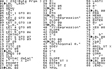
One 41 Program – Three Solutions
Perhaps you are disappointed by my suggestion as it does not benefit from HP-41's distinctive capabilities
to make programs user friendly.
It is a compromise between comfort and size with a bias towards smaller size.
There are options for improvement in either direction, farther squeezed in size or more conveniently
like the following examples.
(Frankly, this program without literals, prompts, printout is my way of Spice series souvenir.
The first RPN calculator I came in touch was a girlfriend's HP-32E.
Probably one of the reasons why I purchased an HP-41C, an enduring source of pleasure,
today again with Orthogonal Regression.)
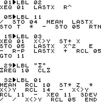 LBL 02 computes $m$ and $b$ for XY-Regression
$m$ is returned in Y and R04, $b$ in X and R05
LBL 11 is for program internal use only.
LBL 03 computes $m$ and $b$ for Orthogonal Regression
$m$ is returned in Y and R04,
$b$ in X and R05
LBL "$\textstyle\sum$" will clear the current statistics data to start a new run
LBL 01 computes $m, b$, and $r$ for YX-Regression
$r$ is returned in Z only,
$m$ in Y and R04, and
$b$ in X and R05
(66 bytes, END comprised)
How to use it
- 1 – XEQ "$\textstyle\sum$"
- Sets start of statistics registers to R10
and clears statistics registers to prepare entering a new set of data points.
The prompt to do so is "DATA ERROR" what is not common practise but saves several bytes.
It's up to you to change that (before LBL 01).
- 2 – data entry/correction
- Accumulating data points with $\scriptstyle\sum+$ and possible correction with $\scriptstyle\sum-$
is described in the "HP-41CX Owner's Manual".
- Now do any of the following steps, in sequence at will:
- — XEQ 01
- Compute $m, b$ and $r$ for L.R.
Except for $r$ the results are saved in registers 04..05 for later use,
see comment for LBL 01 above.
They are also put on the stack, use X<>Y and/or RDN to view either value.
- — XEQ 02
- Computes $m$ and $b$ for XY-Regression.
The results are saved in registers for later use, they are also put on the stack,
see comment for LBL 02 above.
- — XEQ 03
- Computes $m$ and $b$ for Orthogonal Regression.
The results are saved as usual,
see comment for LBL 03 above.
- — data manipulation
- At all times it is possible to go to step 2 to add or correct data. Anyway to #1 too.
Notes:
- The few steps from LBL 03 on comprise all the insight gained by the
calculus shown above.
Same for LBL 02 too.
The rest is well known from users' manuals of several HP pocket calculators,
e.g. "HP-32E Advanced Scientific Calculator Owner's Handbook" (1978), Apendix B, p. 42f.
- The sequence of the program parts is chosen by the purpose to step through using R/S only:
XEQ "$\textstyle\sum$"
– enter data
– R/S for L.R.
– R/S for XY-Regression
– R/S for Orthogonal Regression.
Another R/S now, hit inadvertently, will not erase entered data.
- There are no precautionary measures to prevent overflow, divide by zero, and similar.
I regard such incidents as misuse with faulty input.
- In case the approach of step 1 (purge previous data) is not what you like
and program start should rather re-use ancient remnants,
I suggest to delete line 31.
Even without this modification you may keep previously entered data,
in step 1 shown above,
instead of XEQ use GTO "$\textstyle\sum$" and then continue with any of the following steps.
- It's up to you to enhance the output of the results with literals to be shown in the
display and/or printer, such as here for instance.
- Another complement could be the calculation of linear estimations $\hat{x}$ and $\hat{y}$.
- In addition the labels 01..03 may be replaced by local alpha labels A..C so in user mode
(only in user mode and only if the key in question is not assigned)
a single hit of the corresponding key will start the routine and save prefixing it by XEQ.
- A somewhat more convenient approach ready to use –
NutEm/PC can read the "magnetic cards"
of the following HP67/-97 program and run it.
Same Program on Other Models
HP41 Predecessor and Successor
HP-97 and HP-67
 This program was developed on a virtual HP-97 using
Tony Nixons' stand alone emulator.
Results are printed but it runs also on an HP-67 w/o printer.
This program was developed on a virtual HP-97 using
Tony Nixons' stand alone emulator.
Results are printed but it runs also on an HP-67 w/o printer.
Usage
- 1 - Switch on your HP-97 (or start its emulator)
- Calculators at that time had no 'continuous memory' so switch off and on is a reset to maidenliness.
Note: Only the sliders for printer mode and prgm/run mode may remain set as left at power down.
So before inserting the program card make sure the machine is not in program mode but in run mode.
Otherwise (if the card is not secured) the program on the card may be overwritten what is in most cases
not what you intended.
- 2 - read in program from card
- Run the card through the card reader and place it in the holder above the keys.
So the labels on the card may serve as reminder which function key does now what.
- 3 - hit R/S or Shift a
- After reading the program card the program pointer is on line 1.
So R/S and Shift a do the same, prepare registers for data entry and set flag 0 to enable print.
This sequence ends with Error in the display, remove it with CLX before moving on to next step.
- 4 - data entry
- Data entry with $\scriptstyle\sum+$ and possible correction with $\scriptstyle\sum-$ is described in the
"The HP-97 Programmable Printing Calculator Owner's Handbook and Programming Guide".
- 5 - now it's completely your choice
- If you followed the instructions up to here in sequence you may continue with R/S to run through
functions A - b - B - C.
Or you may press out of sequence any of the function keys as described below.
- A - L.R.
- Compute $m$ and $b$ for Linear Regression (YX-R.)
The results are saved in registers for later use, $m$ in R1 and $b$ in R0, printed ($m$ first) and also
put on the stack, $m$ in Y and $b$ in X.
Use X<>Y and/or RDN to view either value.
- B - XY-Regression
- Computes $m$ and $b$ for XY-Regression.
Results are printed ($m$ first), put on the stack, $m$ in Y and $b$ in X,
and saved in registers, $m$ in R1 and $b$ in R0.
- C - Orthogonal Regression
- Computes $m$ and $b$ for Orthogonal Regression.
Results are printed ($m$ first), put on the stack, $m$ in Y and $b$ in X,
and saved in registers, $m$ in R1 and $b$ in R0.
- b - Correlation Coefficient
- Computes $r$ and prints it.
Result also in X.
- any time - data manipulation
- At all times it is possible to go to step 4 to add or correct data.
- a - clear statistics registers
- To start over with a new data set clear the previous one with Shift a.
HP-42S
 This program was developed on a virtual HP-42S under
Christoph's Emu42.
Results are printed (with literals) if
possible.
This program was developed on a virtual HP-42S under
Christoph's Emu42.
Results are printed (with literals) if
possible.
Usage
- Step 1 – XEQ "LR3K"
- This will start a menu which makes it pretty obvious how to use this program.
- Step 2..n – hit any menu key
- Only $\scriptstyle\sum+$ and $\scriptstyle\sum-$ expect something useful in X and Y, all others just start the indicated routine.
- Step n+1 – hit R/S
- With "b = ..." in the display the execution is halted with program pointer at line 77.
R/S now shows CORR with literal (and prints if enabled and possible).
- Step n+m – EXIT
- At any time hit EXIT to quit the menu system.
Note: indicated program size does not include the END.
Other RPN Models
The simplification of Orthogonal Regression makes it now a candidate also for simple calculators formerly
considered as unsuitable for this task.
Of course, if a machine comes with inbuilt L.R. it is very much advantageous.
HP-10C
This model is very tight in memory.
As program space is shared with registers' storage, the longer a program the less registers are available.
To keep the statistics data and save results impedes lengthy programs.
Following routine computes coefficients for Orthogonal Regression only
and saves them in registers for later use, $m$ in R6, $b$ in R7.
Due to rectangular to polar coordinate conversion
the routine is now short enough so besides $m$ also $b$ can be stored as well
(at last — Whew!).
First version I developed on my
NutEm
Coconut firmware interpreter
(running for sure on one, perhaps on two emulated mainframes and – at minimum –
on one real iron under z/VM 7.2 at that time when I installed it somewhere in Texas).
This youngest update was made with
NutEm/PC.
01-  42  3  L.R.       09-     26  EEX         17-  42  0  MEAN
02-     34  x<>y       10-     30  -	       18-   45 6  RCL 6
03-     36  ENTER^     11-  42 22  R->P	       19-     20  *
04-     40  +	       12-  42 36  Last X      20-     30  -
05-   44 6  STO 6      13-     40  +	       21-   44 7  STO 7
06-  42 48  SDEV       14-   45 6  RCL 6       22-  22 00  RTN
07-     10  /	       15-     10  /	       23-  22 00  RTN
08-  42 11  x^2	       16-   44 6  STO 6
Usage
- Quit programming mode if applicable,
make sure the program pointer is at top of program memory,
- enter/modify statistics data as described in "HP-10C Owner's Handbook",
- hit R/S to compute Orthogonal Regression,
when the program ends w/o error, find $m$ in R6 and Y, $b$ in R7 and X (displayed),
- repeat from step 2 (in case of error from step 1).
HP-12C
In my opinion programming the
HP-12C
is challenging.
Amongst other things it lacks the L.R. but comes with linear estimation, correlation coefficient,
and sample standard deviation what together makes some kind of "halfway L.R.".
Fortunately this machine is not so extreme sparsely equipped with storage as the
a. m. HP-10C.
I developed following routine on my Coconut firmware interpreter.
It computes the coefficients for L.R., XY- and Orthogonal Regression.
*** L.R. ***		*** Orthogonal Regression ***
01-      35  CLX	11-   43 48  SDEV
02-   43  2  Y(X)	12-      10  /
03-      34  X<>Y	13-      36  ENTER^
04-   43 48  SDEV	14-      20  *
05-      10  /		15-      26  EEX
06-      20  *		16-      30  -
07-   44  7  STO 7	17-      36  ENTER^
08-      34  X<>Y	18-      36  ENTER^
09-   44  8  STO 8	19-      20  *
10-      31  R/S	20-   45  7  RCL 7
			21-      36  ENTER^
			22-      40  +
			23-   44  7  STO 7
*** XY-R. ***		24-      36  ENTER^
38-   43 48  SDEV	25-      20  *
39-      10  /		26-      40  +
40-      34  X<>Y	27-   43 21  SQRT
41-   43  1  X(Y)	28-      40  +
42-      33  RDN	29-   45  7  RCL 7
43-43,33 30  GTO 30 --> 30-      10  /
			31-   44  7  STO 7
			32-   43  0  MEAN
			33-   45  7  RCL 7
			34-      20  *
			35-      30  -
			36-   44  8  STO 8
			37-43,33 00  RTN
Usage
All three routines end with $b$ in X and R8, $m$ in Y and R7.
- Make sure the program pointer is at top of program memory, if applicable quit programming mode,
- enter/modify statistics data as described in "hp 12c financial calculator user's guide",
- hit R/S to compute L.R.,
- next R/S will compute Orthogonal Regression,
- repeat from step 2 – or...
- enter GTO 38 and hit R/S to compute XY-Regression,
- repeat from step 2.
Honestly, I found
the basic idea for the L.R. part
years ago on a forum.
What I added besides the two STO is the X<>Y at the end to be in compliance with other
HP-RPN calculators' L.R. function (only AOS models return $m$ in the display register).
HP-32S and -32Sii
Both calculators are equipped with L.R., so my program is just for XY-Regression and Orthogonal Regression.
I developed it on a virtual HP-32Sii under
Christoph's Emu42.
B01 LBL B      C01 LBL C      D01 LBL D
B02 m          C02 m          D02 /
B03 r          C03 ENTER      D03 STO W
B04 x^2        C04 +          D04 y_bar
B05 GTO D      C05 STO Z      D05 x_bar
               C06 sig_y      D06 RCL W
               C07 sig_x      D07 *
               C08 /          D08 -
               C09 x^2        D09 STO Z
               C10 1
               C11 -
               C12 R-P
               C13 LASTx
               C14 +
               C15 RCL Z
Note: before adding more routines put a line D10 RTN to the very end.
Usage
- Enter statistical data as described in "HP 32SII RPN Scientific Calculator Owner's Manual",
- XEQ B for XY-Regression, $b$ in X and Reg Z, $m$ in Y and Reg W,
- XEQ C for Orthogonal Regression, $b$ in X and Reg Z, $m$ in Y and Reg W,
- LBL D is for internal use only (there are no local labels on this machines).
HP-33C
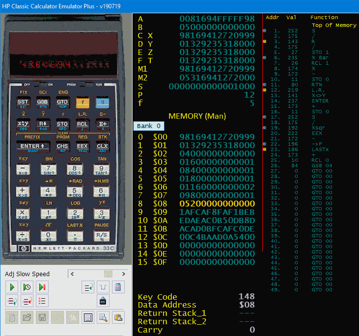 My personal victory: both, XY-Regression and Orthogonal Regression in one routine of
26 bytes only.
Compared with the lengthy and slow HP41 program of my students days this is a big joy.
My personal victory: both, XY-Regression and Orthogonal Regression in one routine of
26 bytes only.
Compared with the lengthy and slow HP41 program of my students days this is a big joy.
Find my routine in adjoined screen shot of Tony Nixons many model running platform
HP Classic Calculator Emulator +.
- Lines 1..11 compute the coefficients for XY-Regression,
- lines 12..26 compute the coefficients for Orthogonal Regression,
- both routines end with $b$ in X and R8, $m$ in Y and R7.
Usage
- Quit programming mode, shift right slider to position RUN if applicable,
- make sure the program pointer is at top of program memory (an OFF-ON sequence will do),
- enter/modify statistics data as described in
"The HP-33E Programmable Scientific Calculator Owner's Handbook and Programming Guide",
- hit R/S to compute XY-Regression,
- hit R/S again to compute Orthogonal Regression,
- repeat from step 3.
Non-RPN Models
HP-22S
This de facto not programmable machine evaluates entered equations and offers
with this feature a simple way to compute user defined formulas.
Alas, it seems there is no option for a "combined result",
so you have to get $m$ first to next get $b$ with it.
Enter your data as mentioned in the "HP-22S Scientific Calculator Owner's Manual",
paragraph "Entering Data for Two-Variable Statistics or Weighted Mean",
then apply the following formulas to compute...
- XY-Regression:
- $\displaystyle m_{XY}=\frac{m_{YX}}{r^2}$;
corresponding equation in HP-22S: M=m/SQ(r)
.
- Orthogonal Regression:
- $m_{OR}=\displaystyle \frac{\sqrt{\left (2m_{YX}\right )^2 + \left ( \left (s_y/s_x\right )^2-1\right )^2} + \left ( \frac{s_y}{s_x} \right )^2 - 1}{2m_{YX}}$;
as equation in 22S: M=(r(2*m:SQ(sy/sx)-1)+SQ(sy/sx)-1)/(2*m)
.
- Ordinate intercept (for both a. m. cases, it is mandatory to compute $m$ first):
- $b=\bar{y}-m\bar{x}$; in 22S: B=$\mathrm{\bar{y}}$-M*$\mathrm{\bar{x}}$
HP-48GX and -50G
To put those calculators here in section "Non-RPN Models" is based on
i) applying power the first time to an HP-50G makes it wakeup in ALG mode, not RPN,
ii) size and location of the Enter key on the HP-50G shows square: this is not an RPN machine,
iii) the LR function returns slope on 1st stack level and y-intercept on 2nd – the way AOS models do it.
All "straight" RPN calculators of HP return y-intercept in X and slope in Y.
This for that.
To compute XY- and Orthogonal Regression I hoped the CAS of the 50G would allow an approach as simple as on the
HP-22S.
Alas, the built-in LR function and typical statistical values are either not accessible from Equation Writer
or I did not find how to do so in the many manuals within reasonable time.
So I may only suggest two RPL routines I developed on an HP-48GX (under
Emu48), which run unchanged also on an
HP-50G.
And (tested now) on a -49G+ too.
- First things first:
- Before running those routines set your machine to RPN mode, enter data as you would for the LR function,
and set it to solve for the Linear Fit model.
The programs base on the slope returned by LR, also on the subroutine
'YINTS', which computes the Y-interception.
.
- Subroutine 'YINTS':
- << ΣY OVER ΣX * - NΣ / >>
.
- XY-Regression:
- << LR SWAP DROP CORR SQ / YINTS "b(XY)" ->TAG SWAP "m(XY)" ->TAG >>
.
- Orthogonal Regression:
- << LR SWAP DROP DUP DUP + SWAP CORR / SQ 1 - DUP2 R->C ABS + SWAP /
YINTS "b(or)" ->TAG SWAP "m(or)" ->TAG >>
Both routines return the results in the same sequence like the LR function
and with literals (tagged) as well.
Other Non-RPN Models
I attempted to double the routines from HP-32Sii on HP-20S and -21S.
It works, it computes the expected figures, alas the programs have 47 and 49 steps.
Thus they lack that lean onward-pace of some of the sleekly RPN counterparts.
I don't feel comfy with AOS, I do not publish those programs.
Conclusion
This refurbished Orthogonal Regression is probably only one example of many
where CAS helps to quicken and to shrink ancient procedures.
So the gain for a single case might be mean to marginal or questionable I have no doubt that CAS is
more than just a toy.
The benefit is the enhanced knowledge that helps for future tasks what will yield in an advantage
on the whole.
What to find in attached ZIP bundle
It contains two directories, HTML with the description and its images you are about to read,
and PRGM with
- OLR.red
- a script to be used with Reduce CAS (Menu/File/Read...) – works also with Web REDUCE
- LR3K.41crm
- a virtual magnetic card to be loaded with the simulated card reader to
NutEm/PC
- LR3K.png
- print out and bar code of that HP41 program, may be used with Software Defined Wand of
NutEm/PC
- linreg.hpp
- a virtual magnetic card to be used with virtual HP-97 or -67 and
NutEm/PC when running an HP41 with CR.
- linreg.bmp
- a picture of that card (when inserted it will be shown by Tony's emulators)
- LR3K-42.RAW
- a program file to be loaded to an HP-42S under Emu42 (Menu/Edit/Load Object...)
- LR-32Sii.RAW
- programs to be loaded to an HP-32Sii under Emu42 (Menu/Edit/Load Object...)
- dcd12cp.rx
- example ooREXX program to analyse the state file of HP's PC version of virtaul 12C
- LR3K for 48GX under Emu48.HP
- directory with programs and example data to be used in HP48GX under Emu48
- LR3K on 49G+ under Emu48+.HP
- same for HP49G+ under Emu48+
- LR3K on 50G under Virt-50G.vobj
- same for HP50G under 'HP Virtual Calculator'
(at least theoretically, at present I'm unable to read it back)
For The Inquisitive
How the program listings made it to this HTML?
There are several ways
because I use virtual calculators only,
from really simple to almost simple:
- clipping of a screen shot, see HP-33C,
- output by inbuilt printer of a virtual HP-97 (contrast-enhanced),
- an HP82240B IR printer simulator,
see HP-42S, HP-48GX and -50G,
- same printer simulator coupled by an
oo82162A IL-to-IR bridge
to virtual HPIL controlled by
Emu41 under DOSBox,
- Show program... option of
NutEm/PC,
see HP-10C and HP-12C,
and for
VM/CMS only:
- analysis of state file content,
see HP-32Sii — Note: this mainframe tool is now
also availabe on PCs,
- my LIF disk dump file content viewer, see here.
The Fine Print
All programs, routines, code snippets, and similar shown in this paper or contained in adjunct ZIP
are published under the following QPL Public License V1.0
THE Q PUBLIC LICENSE version 1.0
Copyright (C) 1999 Trolltech AS, Norway.
Everyone is permitted to copy and
distribute this license document.
The intent of this license is to establish freedom to share and
change the software regulated by this license under the open source
model.
This license applies to any software containing a notice placed by
the copyright holder saying that it may be distributed under the terms
of the Q Public License version 1.0. Such software is herein referred
to as the Software. This license covers modification and distribution
of the Software, use of third-party application programs based on the
Software, and development of free software which uses the
Software.
Granted Rights
1. You are granted the non-exclusive rights set forth in this
license provided you agree to and comply with any and all conditions
in this license. Whole or partial distribution of the Software, or
software items that link with the Software, in any form signifies
acceptance of this license.
2. You may copy and distribute the Software in unmodified form
provided that the entire package, including - but not restricted to -
copyright, trademark notices and disclaimers, as released by the
initial developer of the Software, is distributed.
3. You may make modifications to the Software and distribute your
modifications, in a form that is separate from the Software, such as
patches. The following restrictions apply to modifications:
a. Modifications must not alter or remove any copyright notices in
the Software.
b. When modifications to the Software are released under this
license, a non-exclusive royalty-free right is granted to the initial
developer of the Software to distribute your modification in future
versions of the Software provided such versions remain available under
these terms in addition to any other license(s) of the initial
developer.
4. You may distribute machine-executable forms of the Software or
machine-executable forms of modified versions of the Software,
provided that you meet these restrictions:
a. You must include this license document in the distribution.
b. You must ensure that all recipients of the machine-executable
forms are also able to receive the complete machine-readable source
code to the distributed Software, including all modifications, without
any charge beyond the costs of data transfer, and place prominent
notices in the distribution explaining this.
c. You must ensure that all modifications included in the
machine-executable forms are available under the terms of this
license.
5. You may use the original or modified versions of the Software to
compile, link and run application programs legally developed by you or
by others.
6. You may develop application programs, reusable components and
other software items that link with the original or modified versions
of the Software. These items, when distributed, are subject to the
following requirements:
a. You must ensure that all recipients of machine-executable forms
of these items are also able to receive and use the complete
machine-readable source code to the items without any charge beyond
the costs of data transfer.
b. You must explicitly license all recipients of your items to use
and re-distribute original and modified versions of the items in both
machine-executable and source code forms. The recipients must be able
to do so without any charges whatsoever, and they must be able to
re-distribute to anyone they choose.
c. If the items are not available to the general public, and the
initial developer of the Software requests a copy of the items, then
you must supply one.
Limitations of Liability
In no event shall the initial developers or copyright holders be
liable for any damages whatsoever, including - but not restricted to -
lost revenue or profits or other direct, indirect, special, incidental
or consequential damages, even if they have been advised of the
possibility of such damages, except to the extent invariable law, if
any, provides otherwise.
No Warranty
The Software and this license document are provided AS IS with NO
WARRANTY OF ANY KIND, INCLUDING THE WARRANTY OF DESIGN,
MERCHANTABILITY AND FITNESS FOR A PARTICULAR PURPOSE.
Choice of Law
This license is governed by the laws of most of the remaining members of the European Union (if still existing).
The bottom line of this license is (at least for me), if you are able to improve any of the herein shown
programs, routines, procedures, codes, methods, younameit, you have to inform me about that amendment.
To fulfil this stipulation publish it in an adequate manner just as I did.
And, of course, do not use these programs.
All consequences by disobeying this clause are in full your actual fault.
.....Mike, in October November December 2019
June October 2020 September December 2021
October 2022 November 2023
Changes since first release in October:
HP41 program improved, no "don't forget to XEQ 01 when..." instruction any more,
HP97 program now saves $m$ and $b$ for all three regression variants,
compacted a few algebraic transformations,
put a big thank you in front of all.
Changes since 2nd release in November:
HP41 program same functionality but three bytes tinier, thus a bit faster.
Changes since 3rd release in December:
link to the bundle of virtual HP calculators adjusted.
Changes since 4th release in June:
Reduce is able to show results with indices, added a hint about it,
HP41 program same functionality but one byte less,
adjusted few links, wordings, notes.
Changes since 5th release last year:
Minor adjustments for HP-32Sii as HP-32S is also available in Emu42 now,
added a paragraph about HP-22S because this machine is now emulated too.
Changes since 6th release in September:
Smaller routine for HP-42S,
added RPL-routines for HP-48GX and -50G,
added two..three links,
added a table of contents (kind of).
Changes since 7th release last year:
One..two more hints that
NutEm/PC can read magnetic cards of HP67/-97,
corrected all links to
NutEm/PC.
Changes since 8th release last year:
Editorial revision,
several links adjusted.